Contour plot

Fig.1. Function $f(x,y)=\sin \left({\frac {\pi }{4}}x\right)\sin \left({\frac {\pi }{4}}y\right)$ is plotted in the range $-10\leq x\leq 10~$, $-10\leq y\leq 10~$. Levels $f(x,y)=-0.1$ are shown wiht red lines. Levels $f(x,y)=0.1$ are shown wiht blue lines.

Contour plot is kind of graphical image that shows some function $f(x,y)$ with lines

(1) $f(x,y)=L$,

where $L$ is constant, called level. Such lines are called isolines. If many isolines are shown, their density indicate the slop of the function.

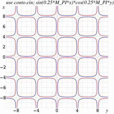
One example of the contour plot is shown in Figure 1. Function $f(x,y)=\sin \left({\frac {\pi }{4}}x\right)\sin \left({\frac {\pi }{4}}y\right)$ is plotted in the range $-10\leq x\leq 10~$, $-10\leq y\leq 10~$. Levels $f(x,y)=-0.1$ are shown wiht red lines. Levels $f(x,y)=0.1$ are shown wiht blue lines.

An isoline actually is graphic of solution of equation (1). One of variables (for example, $x$) can be considered as independent variable, then, another variable can be treated as solution. Graphic of one isoline is called implicit plot. Contour plot can be considered as set of implicit plots, corresponding some sequence of levels.

Countour plots are used to map some surface: relief of the Earth surface at a geographic map, real and imaginary part of a function of complex variable - any bidimensional distribution.

Implementation of contour plot in high level languages

Fig.2. Contour plot of function $f=|z-\ln(z)|$ in the complex $z$-plane, made with Mathematica.

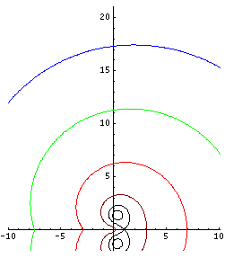
Programming languages of high level (Matlab, Mathematica, Maple) offer the special procedures (operators, "functions") for contour plot and implicit plot. These procedures allow quick programming of contour plots of simple functions (see, for ex., Fig.2 and its source), but may be slow in execution and sometimes do not provide a good compromise between quality of the image and size of the file. Customised codes (like that used to plot Figure 1) may be more efficient, but require some effort for programming.

More examples of contour plots and speculations around can be found at Wikipedia http://en.wikipedia.org/wiki/Contour_plot