Shortest path routing

Shortest path routing refers to the process of finding paths through a network that have a minimum of distance or other cost metric. Routing of data packets on the Internet is an example involving millions of routers in a complex, worldwide, multilevel network. Optimum routing on the Internet has a major impact on performance and cost.

This article will explain a basic routing algorithm that underlies the routing protocols used in small to mid-sized networks. A firm understanding of this algorithm will help in studying those protocols.

The algorithm is presented here in Python, a computer language designed for maximum readability. Computer networks texts often use pseudocode or C to explain algorithms. The problem with pseudocode is it can give you a temporary feeling of understanding, which is lost when you try to actually implement the algorithm. Then you may stumble on the ambiguities you didn't notice in the pseudocode, or find that real programs just don't work that way. The problem with C is that it is too low level. It's great for speed and efficiency, but you may get lost in the details of pointers and indices. You can follow every statement, and still not understand the algorithm. If you are not familiar with Python, see Dijkstra59.py for a more heavily-annotated version of this program, or Dijkstra59.c for the same thing in C.

Figure 1. Computing the shortest path through a network

Figure 1. Computing the shortest path through a network

Figure 2. Time to build routing table using the Python program here

# dijkstra59v05.py              Dijkstra's Algorithm                DMQ 12/23/09
'''
Use Dijkstra's algorithm to compute the shortest paths from a given source node
to all other nodes in a network. Links are bi-directional, with the same
distance in either direction.  Distance can be any measure of cost.
~'''

# Example from Figure 1 (8 nodes, 11 links)
nodeset = {'A', 'B', 'C', 'D', 'E', 'F', 'G', 'H'}

linklist = [('A', 'B', 2), ('B', 'C', 7), ('C', 'D', 3), # (node,node,distance)
            ('B', 'E', 2), ('E', 'F', 2), ('F', 'C', 3),
            ('A', 'G', 6), ('G', 'E', 1), ('G', 'H', 4),
            ('F', 'H', 2), ('H', 'D', 2),               ]

INF = int(1e9)  # larger than any possible path
'''
The strategy is to start at the source node, send probes to each of its adjacent
nodes, pick the node with the shortest path from the source, and make that the
new working node.  Send probes from the new working node, pick the next shortest
path, and make that the next working node.  Continue selecting the shortest
possible path until every every node in the network has been selected.

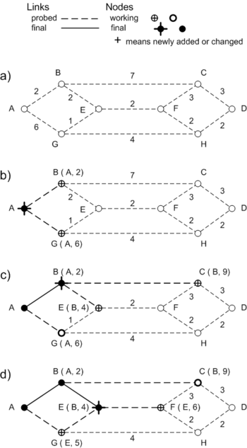
Figure 1 shows the first few steps in our example network. Labels on each node
show its distance from the source, and the previous node on the path from which
that distance was computed.  As new nodes are first probed, they are added to a
working set, shown with a darkened open circle.  After each probe cycle, we look
at the entire set of working nodes.  The node with the shortest path is moved to
a final set, shown with a solid circle.  Figure 1b shows the situation after the
first probes from node 'A', with one node in the final set, and two nodes in the
working set.

The labels on nodes in the working set are tentative.  They will be replaced if
another probe arrives with a shorter total path.  Figure 1d shows node G getting
an update of its label after a probe from node E.  The updates at a node stop
when no other working set node has a shorter path.  This is the proof that the
method works.  The node with the shortest path in a working set can never get
any shorter, because subsequent probes can only come from other working nodes,
and those paths are already at least as long.  There are no negative links.

Figure 1i shows the final tree for node A.  The light dotted lines are links not
used in any shortest path from node A.  They might be used in another tree,
however.  Each node in a network can compute its own shortest path tree, given
the linklist for the entire network.
~'''

def get_LSDB(nodeset, linklist):
    '''Create a Link State Database to quickly look up the adjacent nodes for
any given node.

>>> get_LSDB(nodeset, linklist)
{'A': {('B', 2), ('G', 6)}, 'C': {('B', 7), ('F', 3), ('D', 3)}, \
'B': {('C', 7), ('E', 2), ('A', 2)}, 'E': {('B', 2), ('G', 1), ('F', 2)}, \
'D': {('H', 2), ('C', 3)}, 'G': {('A', 6), ('E', 1), ('H', 4)}, \
'F': {('H', 2), ('E', 2), ('C', 3)}, 'H': {('G', 4), ('D', 2), ('F', 2)}}

    ~'''
    LSDB = {n:set() for n in nodeset} # start with empty set for each node
    for (n1, n2, d) in linklist:
        LSDB[n1].add((n2, d))
        LSDB[n2].add((n1, d))
        
    return LSDB

def build_tree(src, LSDB):
    '''Given a source node and a Link State Database for the network, return a
table with two values for each node - the distance on the shortest path from the
source to that node, and the name of the last node on that path before the final
node.  Saving the previous node makes it easy to re-construct an entire path,
from any leaf to the root of the tree.

>>> build_tree('A', LSDB)
{'A': ('A', 0), 'C': ('B', 9), 'B': ('A', 2), 'E': ('B', 4), \
'D': ('H', 10), 'G': ('E', 5), 'F': ('E', 6), 'H': ('F', 8)}

    ~'''
    # Current working node
    wrk = src
    
    # Nodes in the working set and final set, saved as dictionaries.
    #   {key: value} = {nodename: (previous node, distance from src) }
    Wset = {}; Fset = {}
    Wset[wrk] = (wrk, 0)            # {'A': ('A', 0)}

    while Wset:  # loop until the work set is empty
  
        # Select next wrk node
        dist = INF
        for node in Wset:           # Find the shortest distance in the
            (prev, d) = Wset[node]  # working set, and make that node the
            if d < dist:            # new working node. The distance of that
                dist = d            # node will never get smaller.
                wrk = node
        
        # Move the new working node to the final set.        
        Fset[wrk] = Wset[wrk]
        del Wset[wrk]
        last = wrk                  # last node before end of path

        # Expand the work set
        for (n, d) in LSDB[wrk]:      # Probe the nodes adjacent to wrk      

            new_dist = dist + d          # probe distance
            
            if n in Fset:
                continue                 # skip this node, already finalized
            
            elif (n in Wset) and (new_dist >= Wset[n][1]):
                continue                 # skip this node, probe too long           

            else:  # Add new node to working set, or update existing node
                Wset[n] = (last, new_dist)
    
    return Fset

def build_RT(src, LSDB):
    '''Given a source node and a Link State Database for the network, return a
table with three values for each node - the distance on the shortest path from
the source to that destination node, and the names of the first and last nodes
on the path, not including the endpoints.  The first node is needed in a routing
table.  The last node is needed to construct a tree with src at the root.

>>> build_RT('A', LSDB)
{'A': ('A', 'A', 0), 'C': ('B', 'B', 9), 'B': ('B', 'A', 2), \
'E': ('B', 'B', 4), 'D': ('B', 'H', 10), 'G': ('B', 'E', 5), \
'F': ('B', 'E', 6), 'H': ('B', 'F', 8)}

    ~~'''
    # Current working node
    wrk = src

    # Nodes in the working set and final set, saved as dictionaries.
    #   {key: value} = {nodename: (first, last, distance from src)}
    Wset = {}; Fset = {}

    # Special setup for first step
    Fset[wrk] = (wrk, wrk, 0)      # {'A': ('A', 'A', 0)}
    for (n, d) in LSDB[wrk]:
        first = n                  # first step on the new route
        last = wrk
        Wset[n] = (first, last, d) # {'B': ('B', 'A', 2), 'G': ('G', 'A', 6)}
    
    while Wset:  # loop until the working set is empty
  
        # Select next wrk node
        dist = INF
        for node in Wset:           # Find the shortest distance in the
            (first, last, d) = Wset[node]  # working set, and make that node
            if d < dist:            # the new working node. The distance of
                dist = d            # that node will never get smaller.
                wrk = node
        
        # Move the new working node to the final set        
        Fset[wrk] = Wset[wrk]
        del Wset[wrk]
        # Update first and last hops
        first = Fset[wrk][0]
        last = wrk

        # Expand the work set
        for (n, d) in LSDB[wrk]:      # Probe the nodes adjacent to wrk      

            new_dist = dist + d          # probe distance
            
            if n in Fset:
                continue                 # skip this node, already finalized
            
            elif (n in Wset) and (new_dist >= Wset[n][2]):
                continue                 # skip this node, probe too long           

            else:  # Add new node to working set, or update existing node
                Wset[n] = (first, last, new_dist)
    
    return Fset

Figure 2. Time to build routing table using the Python program here

Limitations

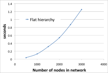
The main limitations of simple shortest-path routing have to do with real-world problems that occur in large networks. We can't just keep adding nodes to a huge routing table at every node. As shown in Figure 2, the time to build (or re-build) a table increases as the square of the number of nodes. Also, as nodes are added, the number of failing links, changes in topology, and other events that trigger re-builds throughout the network - these events will occur more frequently.

Aside from these technical limitations, there are administrative headaches that come with huge networks, and these often set a size limit far short of what is technically possible. A campus-wide network might have 100 nodes with only two connections to the outside world, and no desire to add nodes managed by businesses in the same city. Those businesses might be better served by a city-wide network that includes one of the campus "border" routers. The city-wide network might include a few hundred nodes that all have routing table entries for each other, but only one entry for all the nodes on campus. Similarly, the city network might look like just one node in a larger regional network. Hierarchical routing is one way to partition a network into smaller, more manageable pieces.

A routing algorithm is not enough to design a network. We need a complete routing protocol to deal with real-world issues. The Routing protocol articles will discuss how we handle issues such as:

partitioning - hierarchical is not the only possibility
rapid recovery - minimize the time that the routing tables are "out of sync" with the actual topology
preferential routing - voice packets must not have a noticeable delay
load balancing - don't overload the shortest path
security - keep the bad guys from diverting traffic
policy overrides - block our competitors, even if they are coming through one of our customers